Spatial Queries
-Spatial queries are core to many GIS analysis. The example here demonstrates how to do spatial queries. The question we will try to answer is, ‘Which town centres in Peru are within 10 km of a water source?’.
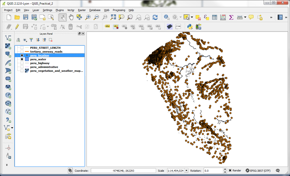
-Load the Vector layers peru_location, which represents town centre information, and peru_water, which represents water sources from the Vector folder, which will be where you originally downloaded and unzipped the files for this practical.
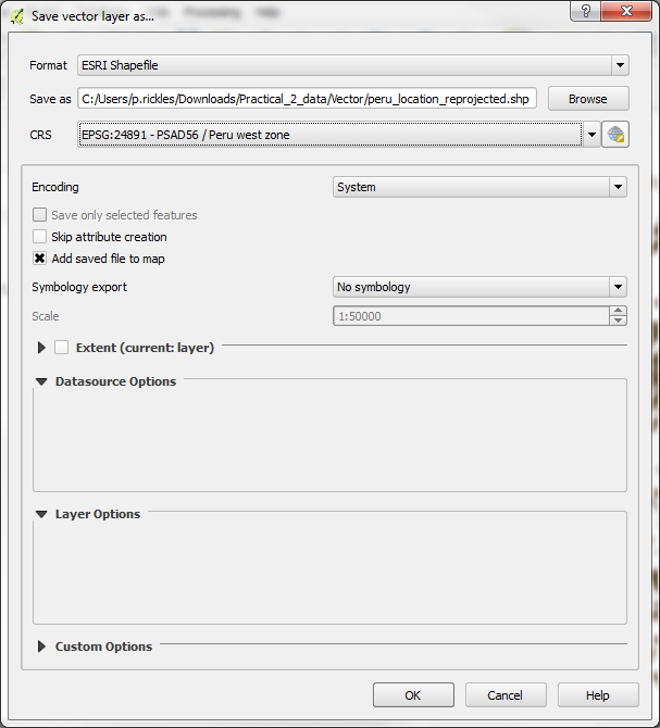
-These layers need to be reprojected to a coordinate system in metres, so we could run our queries in that instead of lat/long. Reprojection is part of the “Save As” menu. This menu can be brought up by right clicking on a layer. In the “Save as” dialog, select PSAD56/Peru west zone as the CRS and save the output file as peru_location_reprojected.shp. Similarly save the other layer as peru_water_reprojected.shp.
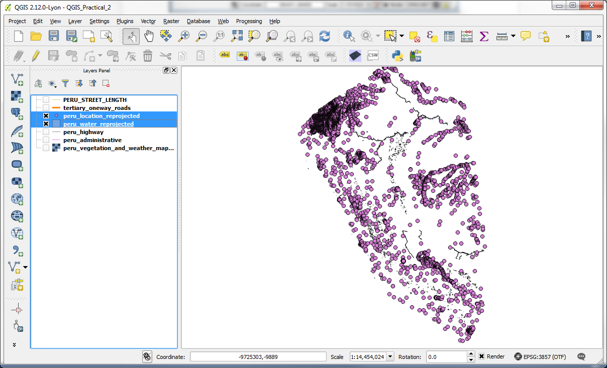
-Once the reprojection is done, the new files should be added to the map as long as the box was ticked to Add saved file to map; if not, add the new files to the map and remove the original peru_water and peru_location layers from project.
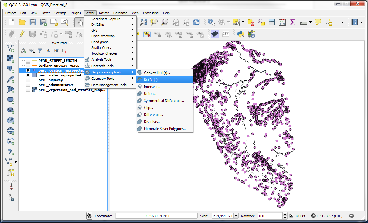
-To answer some spatial queries, further processing of the information may be needed in which we combine datasets or we extract parts common to both datasets (or perhaps the opposite) – this is commonly known as “geoprocessing”. In the next part, we will buffer the existing dataset to highlight information that falls within this proximity; in the Geoprocessing Tools of QGIS, the functions are as follows:
• Convex Hull: Creates the smallest possible convex polygon enclosing a group of objects
• Buffer: Creates an equal zone around specific features at a specified distance
• Intersect: Creates a new layer based on the area of overlap of two layers
• Union: Melds two layers together into one while preserving features and attributes of both
• Symmetrical Difference: Creates a new layer based on areas of two layers that do not overlap
• Clip: Cuts a layer based on the boundaries of another layer
• Difference: Subtracts areas of one layer based on the overlap of another layer
• Dissolve: Merges features within a single layer based on common attributes in the attribute table
(Note: For further information on all of these functions, please review the presentation – Geoprocessing in QGIS)
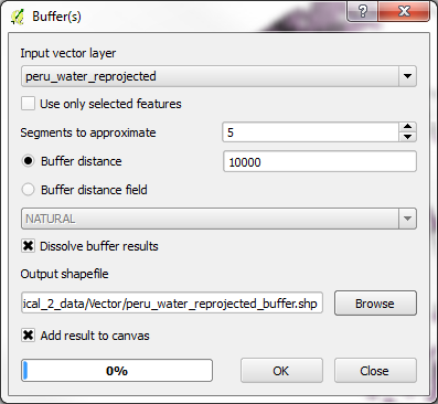
-Now that we are familiar with the terms, we will buffer both the peru_water_reprojected layer by 10,000 metres (10km). Use Vector > Geoprocessing Tools > Buffer for this operation.
-Use 10,000 as the buffer distance since our projection uses metres as units. Click the Dissolve buffer results button so that overlapping buffers are merged and set the Output shapefile to be named peru_water_reprojected_buffer.shp, saved in the folder of your choice.
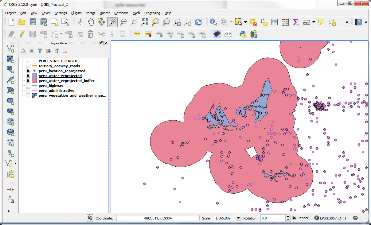
-Once the buffering is done, the layer should have been added to the map as long as you had the box ticked next to Add result to canvas; if not, add the Vector layer from where you saved it.
(Note: you may wish to reorder the layers, change symbology, and/or zoom in a bit to view some of the buffers better.)
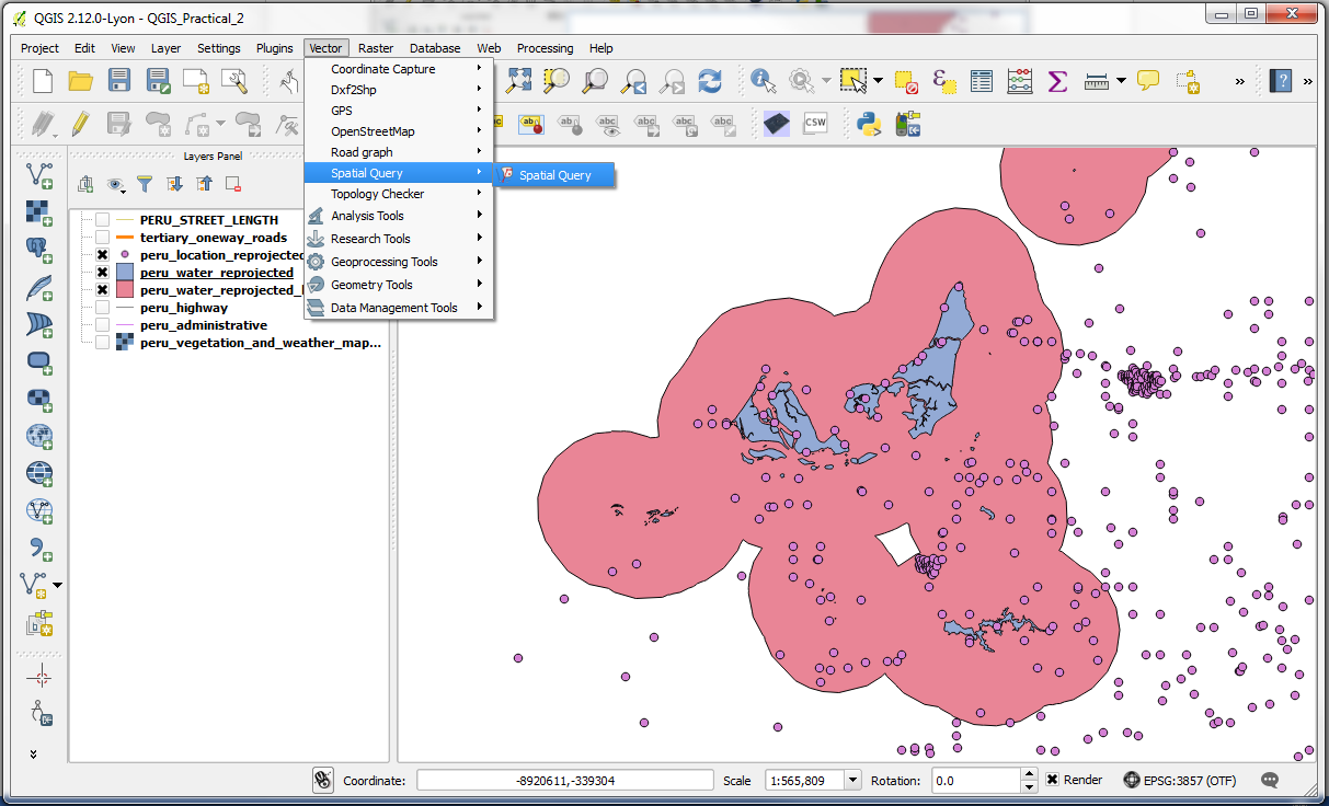
-Now we are ready to run the spatial query to find out our answer to “Which town centres in Peru are within 10km of a water source?”.
-Open the plugin from Vector > Spatial Query.
(Note: You may need to enable it from Plugins > Manage Plugins, if it is not there already.)
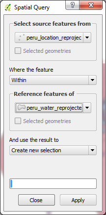
-We want to select all locations that intersect with the buffered water polygon. Select the options as follows:
• Select source features from: peru_location_reprojected
• Where the feature: Within
• Reference features of: peru_water_reprojected_buffer
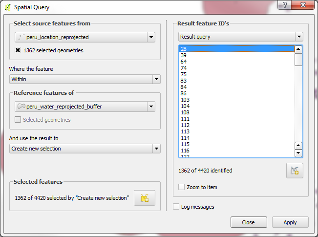
-Click Apply
(Note: the Spatial Query may take some time)
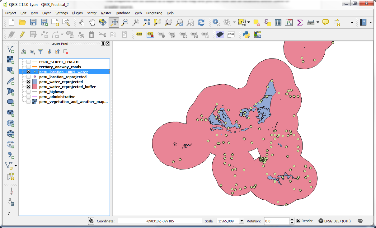
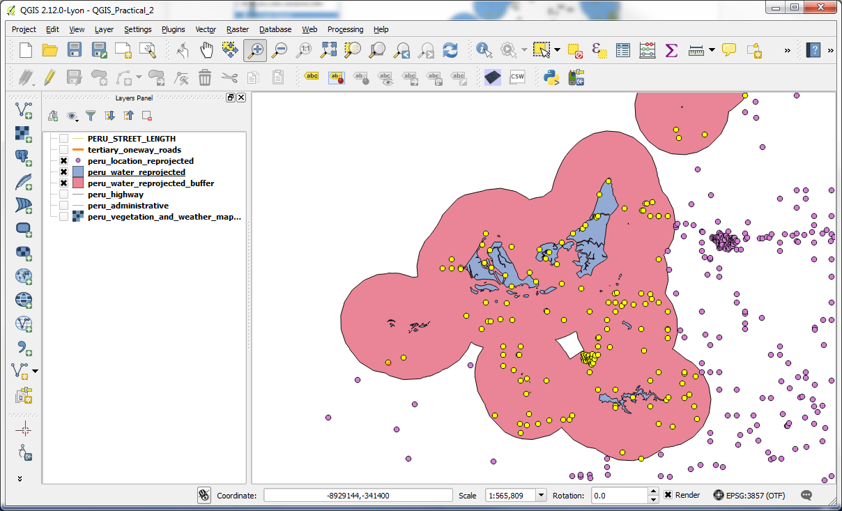
-The new selection will highlight the regions that match the query. This is the answer we are looking for. Click Close and see the highlighted features from the location layer.
-Right-click the peru_location_reprojected layer and save selection, through Save as, as peru_location_10KM_water. Make sure that the boxes next to Save only selected features and Add saved file to map are ticked, then Click OK.
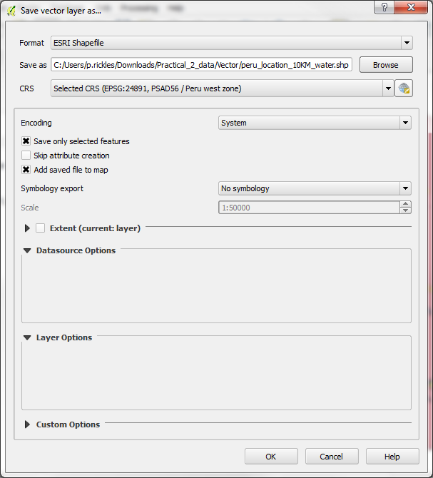
-The shapefile will be added as a layer to the map and you can now see all locations within 10KM of a water source.
(Note: you may need to change the symbology and/or switch layers on/off to better see the new data.)